AEGIS
Adaptive Electromagnetic Geometric Illumination & Safety
AEGIS computes absorbed power density on human body surfaces in wireless environments. It replaces volumetric EM simulation (\(10^{12}\) voxels) with \(O(MN)\) surface operations by exploiting the geometric nature of mmWave dosimetry.
The core equation:
Nine fidelity levels (0-8) provide a controlled accuracy-cost tradeoff, from \(O(1)\) worst-case bounds to \(O(M_{\mathrm{ant}}^3)\) exposure-constrained beamforming.
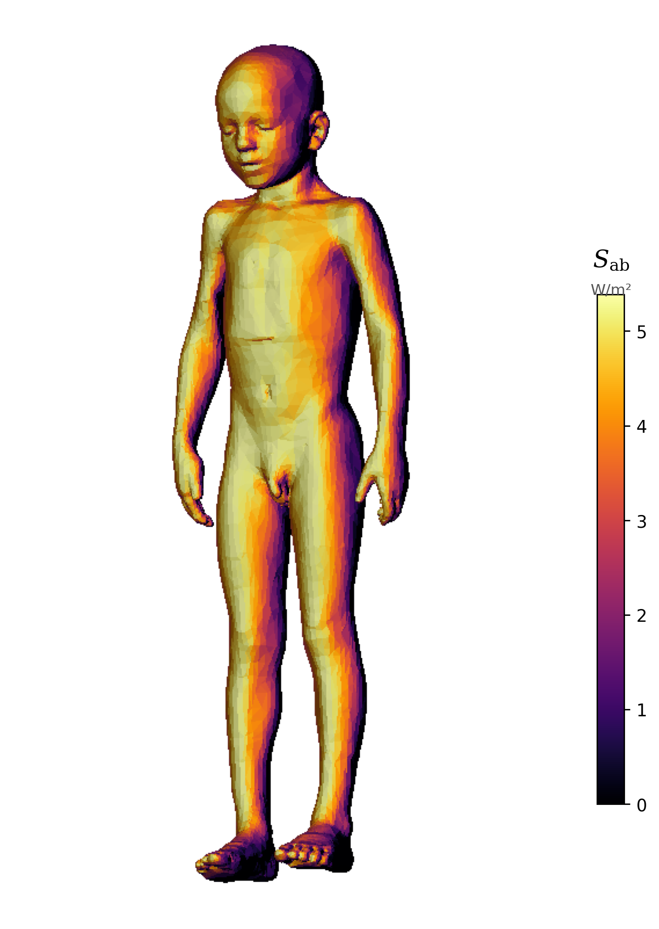
-
Getting started
Install AEGIS and run your first dosimetry computation in under a minute.
-
Fidelity levels
Nine levels from worst-case bounds to coherent MIMO beamforming.
-
Tissue and geometry
Cole-Cole dielectric models, Fresnel transmission, and body mesh operations.
-
API reference
Auto-generated from source. Every public class and function documented.
-
Architecture
Module structure, data flow, and design principles.
-
Testing
Golden tests, property tests, Mie regression, and 260+ test cases.
Quick start
from aegis import DosimetryEngine, BodyMesh, TissueModel, PropagationPaths

skin = TissueModel.from_database("Skin", 28e9)
body = BodyMesh.load("thelonious.stl")
paths = PropagationPaths.from_powers(k_hat=[[0, 0, -1]], power=[1.0])

engine = DosimetryEngine(skin)
result = engine.compute(body, paths, level=2)

print(f"P_abs = {result.p_abs:.4f} W")
print(f"Peak S_ab = {result.peak_sab:.2f} W/m²")
How it works
AEGIS treats the human body as a triangle mesh and incoming wireless signals as propagation paths (directions + powers). For each triangle, the kernel computes absorbed power density based on the angle between the surface normal and the incoming wave direction.
The key insight: at mmWave frequencies, the skin depth is so shallow (< 0.5 mm) that absorption is entirely a surface phenomenon. This makes the \(O(MN)\) geometric computation exact to within 0.35% of the full Fresnel solution.
Fidelity levels at a glance
| Level | Name | What it adds | Cost |
|---|---|---|---|
| 0 | Bound | Worst-case \(P_{\mathrm{abs}}\) | \(O(1)\) |
| 1 | Aggregate | SH-compressed directivity | \(O(L^2)\) |
| 2 | Geometric | ReLU kernel on mesh | \(O(MN)\) |
| 3 | Fresnel | Angle-dependent \(T(\theta)\) | \(O(MN)\) |
| 4 | Polarisation | TE/TM decomposition | \(O(MN)\) |
| 5 | Curvature | Local curvature correction | \(O(MN)\) |
| 6 | Diffraction | GELU shadow smoothing | \(O(MN)\) |
| 7 | Coherent | Complex field summation | \(O(MNK)\) |
| 8 | ECBF | Exposure-constrained beamforming | \(O(K^3)\) |
In practice, all nine levels complete in milliseconds for typical meshes. Pick the level that matches your physics requirements, not your performance budget.