Tutorial 5: Coherent MIMO and ECBF
This tutorial covers fidelity levels 7 and 8: coherent MIMO dosimetry and exposure-constrained beamforming (ECBF). You will build a multi-element channel, compute absorbed power density with a matched beamformer, inspect the exposure operator \(Q\), and then solve the QCQP to find the precoder that maximizes signal power while keeping absorbed power below an ICNIRP limit.
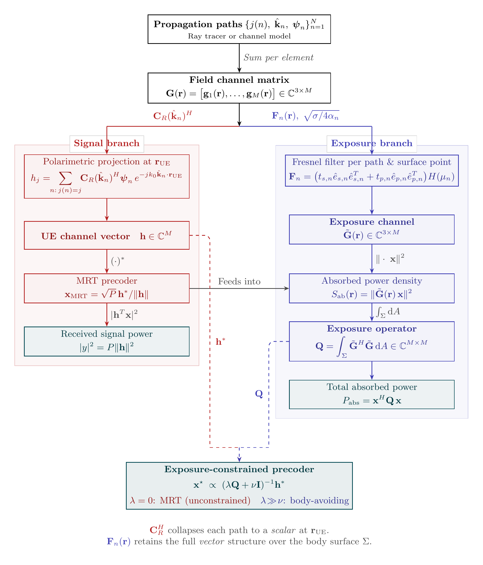
Signal branch (red) and exposure branch (blue) of the coherent MIMO pipeline.
Why coherent matters
Incoherent kernels (levels 0-6) treat each propagation path as an independent power contribution. They sum scalar powers and cannot represent the interference pattern produced by a phased array. Coherent kernels operate on complex polarisation-amplitude vectors \(\boldsymbol{\psi}_n \in \mathbb{C}^3\) and a complex precoding vector \(\mathbf{x} \in \mathbb{C}^{M_{\mathrm{ant}}}\).
The absorbed power density at surface point \(\mathbf{r}\) is:
where \(\tilde{G}(\mathbf{r}) \in \mathbb{C}^{3 \times M_{\mathrm{ant}}}\) is the body-surface channel matrix, which folds in the Fresnel transmission operator and depth-coupling weights. Total absorbed power integrates over the surface:
\(Q \in \mathbb{C}^{M_{\mathrm{ant}} \times M_{\mathrm{ant}}}\) is Hermitian positive semi-definite by construction. Its eigenvalues reveal the absorption modes of the array-body system. The maximum eigenvalue \(\lambda_{\max}\) gives the worst-case absorbed power for any unit-power precoder.
Setup
import numpy as np
import matplotlib.pyplot as plt
import scienceplots  # noqa: F401
plt.style.use(["science", "ieee", "no-latex"])
plt.rcParams.update({"figure.figsize": (3.5, 2.625)})

from aegis import DosimetryEngine
from aegis import BodyMesh, PropagationPaths, TissueModel
from aegis.tissue.dielectric import SKIN_28GHZ
from aegis.precoder import Precoder
from aegis.coherent import (
    compute_body_channel,
    compute_exposure_operator,
    compute_field_channel,
    compute_rho,
    eigendecompose_Q,
    solve_ecbf,
)
Body mesh and tissue
Use a sphere as a simplified phantom and skin tissue at 28 GHz. The predefined SKIN_28GHZ constant has \(\varepsilon_r = 17.0\), \(\sigma = 25.0\) S/m.
body = BodyMesh.sphere(radius=0.1, n_subdivisions=3)
tissue = SKIN_28GHZ
freq_hz = tissue.freq_hz  # 28e9 Hz

print(f"Mesh: {body.n_triangles} triangles")
print(f"T0 = {tissue.T0:.4f}, sigma = {tissue.sigma} S/m")
Building coherent paths
PropagationPaths stores complex polarisation-amplitude vectors \(\boldsymbol{\psi}_n\) (units: V/m per sqrt(W)) and an element_index array that maps each path to its originating antenna element. This structure is what distinguishes a coherent channel from a scalar-power incoherent one.
Here a 4-element uniform linear array (ULA) illuminates the body with 12 paths: 3 per element, arriving from different directions. Real deployments would obtain these from a ray tracer (see aegis.integration).
M_ant = 4   # antenna elements
N = 12      # total paths (3 per element)
rng = np.random.default_rng(42)

# Random arrival directions, normalised
k_hat_raw = rng.standard_normal((N, 3))
k_hat = k_hat_raw / np.linalg.norm(k_hat_raw, axis=1, keepdims=True)

# Complex polarisation-amplitude vectors: |psi|^2 / (2*Z0) = power
# Amplitude chosen to give ~1 W/m^2 average incident power per path
Z0 = 376.73
amplitude = np.sqrt(2 * Z0 * 1.0)
psi_raw = rng.standard_normal((N, 3)) + 1j * rng.standard_normal((N, 3))
psi = amplitude * psi_raw / np.linalg.norm(psi_raw, axis=1, keepdims=True)

# Assign paths to elements: 3 paths each
element_index = np.repeat(np.arange(M_ant), N // M_ant).astype(np.intp)

paths = PropagationPaths(
    k_hat=k_hat,
    psi=psi,
    element_index=element_index,
    delay=np.zeros(N, dtype=np.float64),
    is_los=np.ones(N, dtype=bool),
)

print(paths)  # PropagationPaths(n_paths=12, n_elements=4)
The delay and is_los fields are metadata used by ray tracers and optional filtering. They do not affect the dosimetry kernels.
UE channel vector
Level 8 (ECBF) and the MRT precoder both require a UE channel vector \(\mathbf{h} \in \mathbb{C}^{M_{\mathrm{ant}}}\). This vector represents the signal channel from each antenna element to the user equipment. In a simulation, build it by summing the path contributions at a reference receive point.
# Reference receive point 1 m from the body centroid
r_rx = np.array([1.0, 0.0, 0.0])
k0 = 2 * np.pi * freq_hz / 3e8

# h_j = sum of psi_n * exp(-i k0 k_hat_n . r_rx) for paths n from element j
h = np.zeros(M_ant, dtype=complex)
for j in range(M_ant):
    mask = element_index == j
    phases = np.exp(-1j * k0 * (k_hat[mask] @ r_rx))
    h[j] = np.sum((psi[mask] * phases[:, None])[:, 0])  # take x-component

print(f"h shape: {h.shape}, ||h|| = {np.linalg.norm(h):.4f}")
Level 7: coherent beamforming with MRT
Maximum ratio transmission (MRT) maximises received signal power at the UE. The precoder is \(\mathbf{x} = \sqrt{P}\,\mathbf{h}^* / \|\mathbf{h}\|\). Call Precoder.mrt() with the channel vector and the total transmit power in watts.
P_tx = 1.0  # total transmit power [W]
precoder_mrt = Precoder.mrt(h, P=P_tx)
print(precoder_mrt)  # Precoder(M=4, P=1.0000 W)
Pass the precoder to engine.compute() with level=7. The engine also accepts h at level 7, which it uses to compute the exposure metric \(\rho\) (see below). Omit h if you only need \(S_{\mathrm{ab}}\) and \(P_{\mathrm{abs}}\).
engine = DosimetryEngine(tissue)

result_mrt = engine.compute(
    body,
    paths,
    level=7,
    precoder=precoder_mrt,
    h=h,
    freq_hz=freq_hz,
)

print(f"Peak S_ab  = {result_mrt.peak_sab:.4f} W/m^2")
print(f"P_abs      = {result_mrt.p_abs:.6f} W")
print(f"rho        = {result_mrt.rho:.4f}")
result_mrt.sab is an (M,) array of per-triangle absorbed power density in W/m^2. result_mrt.p_abs is the integral \(\mathbf{x}^H Q \mathbf{x}\) over the mesh.
Exposure operator Q
The level 7 result carries result_mrt.Q, the \(M_{\mathrm{ant}} \times M_{\mathrm{ant}}\) exposure operator computed during the kernel run. It is Hermitian by construction. Verify this and inspect its eigenspectrum.
Q = result_mrt.Q
print(f"Q shape: {Q.shape}")

# Hermitian check: Q - Q^H should be near zero
hermitian_residual = np.max(np.abs(Q - Q.conj().T))
print(f"Hermitian residual: {hermitian_residual:.2e}")

# Eigendecomposition (eigenvalues in descending order)
eigenvalues, eigenvectors = eigendecompose_Q(Q)
print(f"Eigenvalues: {np.real(eigenvalues)}")
print(f"lambda_max = {eigenvalues[0]:.4f}")
The eigenvalues are real and non-negative (numerical noise is clamped to zero by eigendecompose_Q). The engine also returns result_mrt.eigenvalues directly, so you do not need to call eigendecompose_Q again if the result is already in hand.
Rho: exposure-signal alignment
\(\rho\) measures how aligned the signal channel is with the dominant absorption mode of the array:
A value near 1 means MRT beamforming is also directing power into the body's highest-absorption mode. A value near 0 means the signal and absorption modes are nearly orthogonal, so you can beamform toward the UE with little absorbed power. The metric is computed automatically at level 7 when h is provided, and stored in result.rho.
# Verify against the standalone function
rho_check = compute_rho(h, Q, lambda_max=float(np.real(eigenvalues[0])))
print(f"rho from result:   {result_mrt.rho:.4f}")
print(f"rho from function: {rho_check:.4f}")
Eigenspectrum visualization
The eigenspectrum shows how many effective spatial modes contribute to absorption. A fast-decaying spectrum means one or two array directions dominate exposure.
fig, ax = plt.subplots(figsize=(3.5, 2.0))
indices = np.arange(1, M_ant + 1)
ax.bar(indices, np.real(eigenvalues), width=0.6)
ax.set_xlabel("Eigenvalue index")
ax.set_ylabel(r"$\lambda_i$ (W$\cdot$m$^2$ / (V/m)$^2$)")
ax.set_xticks(indices)
plt.show()
Level 8: ECBF
Level 8 solves the exposure-constrained beamforming (ECBF) QCQP:
The optimal solution scales the MRT precoder by \((\lambda Q + \nu I)^{-1}\) in the eigenbasis of \(Q\), where \(\lambda\) and \(\nu\) are Lagrange multipliers found by bisection. When the MRT precoder already satisfies the constraint, the solution reduces to MRT.
The ICNIRP 2020 general-public \(S_{\mathrm{ab}}\) limit over 4 cm^2 is 20 W/m^2. Convert it to a total absorbed power budget using the body surface area as a rough scaling (actual ECBF operates on \(P_{\mathrm{abs}}\), not \(S_{\mathrm{ab}}\) directly):
# Example budget: allow at most 50 mW absorbed by the body
P_abs_max = 0.05  # W

result_ecbf = engine.compute(
    body,
    paths,
    level=8,
    h=h,
    P_abs_max=P_abs_max,
    freq_hz=freq_hz,
)

print(f"ECBF peak S_ab = {result_ecbf.peak_sab:.4f} W/m^2")
print(f"ECBF P_abs     = {result_ecbf.p_abs:.6f} W  (budget: {P_abs_max} W)")
print(f"ECBF rho       = {result_ecbf.rho:.4f}")

# Retrieve the optimal precoder vector
x_star = result_ecbf.x_star
print(f"||x_star||^2   = {np.real(np.vdot(x_star, x_star)):.4f} W")
result_ecbf.x_star is the \(M_{\mathrm{ant}}\)-dimensional optimal precoding vector. Its squared norm equals the transmit power budget \(P\).
Comparing MRT and ECBF
sig_mrt  = abs(h.conj() @ precoder_mrt.x) ** 2
sig_ecbf = abs(h.conj() @ x_star) ** 2

print(f"{'Metric':<20} {'MRT':>12} {'ECBF':>12}")
print("-" * 46)
print(f"{'Peak S_ab (W/m^2)':<20} {result_mrt.peak_sab:>12.4f} {result_ecbf.peak_sab:>12.4f}")
print(f"{'P_abs (W)':<20} {result_mrt.p_abs:>12.6f} {result_ecbf.p_abs:>12.6f}")
print(f"{'rho':<20} {result_mrt.rho:>12.4f} {result_ecbf.rho:>12.4f}")
print(f"{'Signal power':<20} {sig_mrt:>12.4f} {sig_ecbf:>12.4f}")
ECBF trades signal power for absorption reduction. The gap between sig_mrt and sig_ecbf depends on \(\rho\): when \(\rho \approx 0\), signal and absorption modes are nearly orthogonal and ECBF incurs almost no signal penalty.
Direct use of the building-block functions
The kernel functions are accessible without going through DosimetryEngine. Use these for custom optimization loops or differentiable (JAX) workflows.
Body-surface channel \(\tilde{G}(\mathbf{r})\), incorporating Fresnel transmission and depth coupling:
G_tilde = compute_body_channel(
    normals=body.normals,
    centroids=body.centroids,
    k_hat=paths.k_hat,
    psi=paths.psi,
    element_index=paths.element_index,
    n_tilde=tissue.n_complex,
    sigma=tissue.sigma,
    freq_hz=freq_hz,
    n_elements=M_ant,
)
print(f"G_tilde shape: {G_tilde.shape}")  # (M_tri, 3, M_ant)
Field channel \(G(\mathbf{r})\), the raw phase-coherent field without Fresnel filtering:
G = compute_field_channel(
    centroids=body.centroids,
    k_hat=paths.k_hat,
    psi=paths.psi,
    element_index=paths.element_index,
    freq_hz=freq_hz,
    n_elements=M_ant,
)
print(f"G shape: {G.shape}")  # (M_tri, 3, M_ant)
Exposure operator from G_tilde:
Q_direct = compute_exposure_operator(G_tilde, body.areas)
print(f"Q_direct shape: {Q_direct.shape}")  # (M_ant, M_ant)
Solve ECBF directly, without the engine:
x_opt = solve_ecbf(h, Q_direct, P_abs_max=0.05, P=1.0)
P_abs_check = float(np.real(x_opt.conj() @ Q_direct @ x_opt))
print(f"Direct solve: P_abs = {P_abs_check:.6f} W")
Compliance for coherent results
DosimetryResult.evaluate_compliance() runs a full ICNIRP 2020 check. Spatial averaging over 4 cm^2 is computed automatically (unless you passed spatial_averaging=False).
from aegis.compliance import ExposureScenario, summary_text

compliance_mrt  = result_mrt.evaluate_compliance(ExposureScenario.GENERAL_PUBLIC)
compliance_ecbf = result_ecbf.evaluate_compliance(ExposureScenario.GENERAL_PUBLIC)

print("--- MRT ---")
print(summary_text(compliance_mrt))

print("--- ECBF ---")
print(summary_text(compliance_ecbf))
ComplianceResult.overall_pass is True if every available check passes. ComplianceResult.margin_db gives the tightest margin across all checks. A positive margin means compliant, negative means exceeded.
Scaling and power sweeps
DosimetryResult.scale() rescales all power quantities without re-running the kernel. This is useful for finding the maximum compliant transmit power:
from aegis.compliance import max_compliant_power

# Find maximum compliant TX power given the MRT result at 1 W
p_max = max_compliant_power(compliance_mrt, ref_power_w=P_tx)
print(f"Max compliant TX power (MRT): {p_max * 1e3:.2f} mW")

result_scaled = result_mrt.scale(p_max / P_tx)
compliance_scaled = result_scaled.evaluate_compliance()
print(f"At max power, margin = {compliance_scaled.margin_db:+.2f} dB")
Next steps
- Replace the random channel with a ray-traced one using
aegis.integrationand DiffeRT. - Use
jax.gradthroughengine.compute_sab(..., level=7)to optimize \(\mathbf{h}\) or array placement. - See the compliance module for
power_sweep()andcompliance_heatmap()to explore the transmit power envelope. - Fidelity levels 5-6 add curvature and diffraction corrections. Run both and use
DosimetryResult.compare()to quantify the error from omitting them.