Tutorial 2: Fidelity levels and convergence
AEGIS organises its physics models into nine fidelity levels (0-8). Higher levels add physics corrections at increasing computational cost. This tutorial shows how each level affects computed \(S_{\mathrm{ab}}\), how to run a convergence sweep, and how many paths you need for a stable estimate.
The three-tier hierarchy
The nine levels fall into three tiers based on what they compute. The cost column shows theoretical scaling, but all levels run in milliseconds for typical meshes. The real selection criterion is which physics corrections your scenario requires.
| Tier | Levels | Cost | Output |
|---|---|---|---|
| Bound | 0 | \(O(1)\) | Scalar \(P_{\mathrm{abs}}\) upper bound, uniform \(S_{\mathrm{ab}}\) |
| Aggregate | 1 | \(O(N)\) | Scalar \(P_{\mathrm{abs}}\) weighted by directivity, uniform \(S_{\mathrm{ab}}\) |
| Spatial | 2-6 | \(O(MN)\) | Per-triangle \(S_{\mathrm{ab}}(\mathbf{r})\) map with progressive corrections |
| Coherent | 7-8 | \(O(M \cdot M_{\mathrm{ant}}^2)\) | Per-triangle \(S_{\mathrm{ab}}\) from complex field superposition |
\(M\) = number of body triangles, \(N\) = number of propagation paths, \(M_{\mathrm{ant}}\) = number of antenna elements.
Levels 0 and 1 require precomputed antenna parameters (\(A_{\mathrm{ab}}\) and \(D_{\mathrm{max}}\)) that are not always available. Levels 2-6 need only the body mesh, tissue model, and a set of propagation paths. Coherent levels 7-8 require per-path complex amplitudes and are covered in Tutorial 5.
Spatial levels 2-6 in detail
Each level adds one physical correction on top of the previous one.
| Level | Correction added | Key equation |
|---|---|---|
| 2 | Geometric ReLU with constant \(T_0\) | \(S_{\mathrm{ab}} = T_0 \cdot [\hat{n} \cdot (-\hat{k})]_+ \cdot S_{\mathrm{inc}}\) |
| 3 | Angle-dependent Fresnel \(T(\theta_i)\) | \(T_0 \to T_{\mathrm{avg}}(\theta_i)\) |
| 4 | Polarisation correction | \(T_{\mathrm{avg}} \to T_{\mathrm{avg}} + \tfrac{q}{2} \Delta T\) |
| 5 | Surface curvature (Physical Optics) | adds \(T_0 \cdot \frac{H}{k} \cdot g(\mu)^2 \cdot S_{\mathrm{inc}}\) |
| 6 | Diffraction smoothing | replaces ReLU with GELU at shadow boundaries |
Level 3 is the default when you call engine.compute(body, paths, mode="spatial"). The Fresnel correction alone reduces the error from a constant-\(T_0\) assumption by roughly 5.6% for skin at 28 GHz.
Setup
These imports and helpers are shared across all code blocks in this tutorial.
import numpy as np
import matplotlib.pyplot as plt
import scienceplots  # noqa: F401
plt.style.use(["science", "ieee", "no-latex"])
plt.rcParams.update({"figure.figsize": (3.5, 2.625)})

from aegis import DosimetryEngine, BodyMesh, PropagationPaths
from aegis.tissue.dielectric import SKIN_28GHZ

# Icosahedron: 20 triangles, 10 cm radius, outward normals
phi = (1 + np.sqrt(5)) / 2
verts_raw = np.array([
    [-1, phi, 0], [1, phi, 0], [-1, -phi, 0], [1, -phi, 0],
    [0, -1, phi], [0, 1, phi], [0, -1, -phi], [0, 1, -phi],
    [phi, 0, -1], [phi, 0, 1], [-phi, 0, -1], [-phi, 0, 1],
], dtype=float)
verts_raw /= np.linalg.norm(verts_raw[0])
verts_raw *= 0.1  # 10 cm radius

faces = [
    (0,11,5),(0,5,1),(0,1,7),(0,7,10),(0,10,11),
    (1,5,9),(5,11,4),(11,10,2),(10,7,6),(7,1,8),
    (3,9,4),(3,4,2),(3,2,6),(3,6,8),(3,8,9),
    (4,9,5),(2,4,11),(6,2,10),(8,6,7),(9,8,1),
]
n_tri = len(faces)
vertices = np.zeros((n_tri, 3, 3))
for i, (a, b, c) in enumerate(faces):
    vertices[i] = [verts_raw[a], verts_raw[b], verts_raw[c]]

v0, v1, v2 = vertices[:, 0], vertices[:, 1], vertices[:, 2]
cross = np.cross(v1 - v0, v2 - v0)
lens = np.linalg.norm(cross, axis=1, keepdims=True)
normals = cross / lens
centroids = vertices.mean(axis=1)
# Flip inward-pointing normals
flip = np.einsum("ij,ij->i", normals, centroids) < 0
normals[flip] *= -1
areas = 0.5 * lens[:, 0]

body = BodyMesh(
    vertices=vertices,
    normals=normals,
    centroids=centroids,
    areas=areas,
    name="icosahedron",
)

# 50 random paths, uniform directions, equal power
rng = np.random.default_rng(42)
N = 50
k_hat = rng.standard_normal((N, 3))
k_hat /= np.linalg.norm(k_hat, axis=1, keepdims=True)
power = np.ones(N) * 10.0  # 10 W/m^2 each

paths = PropagationPaths.from_powers(k_hat=k_hat, power=power)

engine = DosimetryEngine(SKIN_28GHZ)
Level 2 baseline
Level 2 uses the geometric ReLU with the constant normal-incidence transmission coefficient \(T_0\).
result2 = engine.compute(body, paths, level=2)

print(f"Level 2  P_abs = {result2.p_abs:.4f} W")
print(f"         T0    = {SKIN_28GHZ.T0:.4f}")
print(f"         S_ab  mean = {result2.sab.mean():.4f} W/m^2")
print(f"         S_ab  max  = {result2.sab.max():.4f} W/m^2")
The output confirms that some triangles receive no power (shadowed faces where \(\hat{n} \cdot (-\hat{k}) \le 0\)) and illuminated faces get a cosine-weighted sum.
Level 3: angle-dependent Fresnel
Level 3 replaces \(T_0\) with the angle-averaged Fresnel transmission \(T_{\mathrm{avg}}(\theta_i)\), evaluated at the angle of incidence for each path. The difference is significant near grazing angles where \(T_{\mathrm{avg}}\) rises above \(T_0\) due to the TM pseudo-Brewster effect.
result3 = engine.compute(body, paths, level=3)

print(f"Level 3  P_abs = {result3.p_abs:.4f} W")
delta = (result3.p_abs - result2.p_abs) / result2.p_abs * 100
print(f"         change from level 2: {delta:+.2f}%")
For skin at 28 GHz with isotropic paths the correction is typically a few percent. In scenarios with predominantly grazing arrivals it can exceed 10%.
Sweep all incoherent levels
sweep_levels runs all specified levels in one call and returns a dict mapping level to result. Levels 0 and 1 require A_ab and D_max. If those are not provided, sweep_levels silently skips those levels.
# Levels 2-6 need no extra parameters for this synthetic example
results = engine.sweep_levels(body, paths, levels=[2, 3, 4, 5, 6])

print(f"{'Level':>6}  {'P_abs (W)':>12}  {'S_ab mean (W/m^2)':>18}  {'S_ab max (W/m^2)':>17}")
print("-" * 62)
for lvl, res in sorted(results.items()):
    print(f"{lvl:>6}  {res.p_abs:>12.5f}  {res.sab.mean():>18.5f}  {res.sab.max():>17.5f}")
To include levels 0 and 1 you need antenna parameters from a body-specific calculation (see Tutorial 4). Providing them is straightforward:
# Example with antenna parameters (replace with actual values)
A_ab = 1.2e-3   # absorption area in m^2
D_max = 3.0     # maximum directivity (dimensionless)

results_all = engine.sweep_levels(
    body, paths,
    levels=[0, 1, 2, 3, 4, 5, 6],
    A_ab=A_ab,
    D_max=D_max,
)
Mode-based API
The mode API makes the corrections explicit without memorising level numbers. All combinations below are equivalent to the corresponding integer levels.
# Level 2: spatial kernel, no Fresnel
r = engine.compute(body, paths, mode="spatial", fresnel=False)

# Level 3: spatial kernel with Fresnel (default when mode="spatial")
r = engine.compute(body, paths, mode="spatial")
r = engine.compute(body, paths, mode="spatial", fresnel=True)  # same

# Level 4: add polarisation correction (requires per-path TM excess q)
q = rng.uniform(-1, 1, size=N)   # TM excess in [-1, 1] per path
r = engine.compute(body, paths, mode="spatial", polarisation=True, q=q)

# Level 5: curvature correction (requires per-triangle twice-mean curvature H)
H = np.zeros(body.n_triangles)   # flat approximation: H = 0
r = engine.compute(body, paths, mode="spatial", curvature=True, curvature_H=H)

# Level 6: diffraction smoothing (enables curvature implicitly)
r = engine.compute(body, paths, mode="spatial", diffraction=True, curvature_H=H)
The mode API is preferable when you want composable corrections without coupling to the integer level numbering. result.fidelity_level and result.corrections record what was actually computed.
Multipath convergence
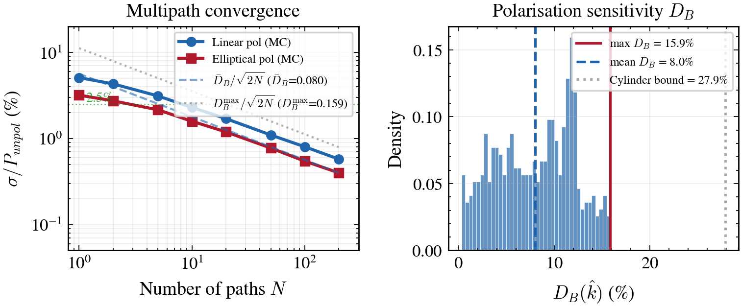
Convergence of \(P_{\mathrm{abs}}\) error with number of paths \(N\), with theoretical \(O(1/\sqrt{N})\) bounds.
The incoherent absorbed power density converges as paths are added. For \(N\) independent paths the standard error of the mean decays as \(1/\sqrt{N}\). The Cauchy convergence criterion compares consecutive estimates:
n_values = [5, 10, 20, 50, 100, 200, 500]
p_abs_values = []

# Generate a large pool of paths; subsample for each N
rng2 = np.random.default_rng(0)
N_max = max(n_values)
k_pool = rng2.standard_normal((N_max, 3))
k_pool /= np.linalg.norm(k_pool, axis=1, keepdims=True)
p_pool = np.ones(N_max) * 10.0

for n in n_values:
    paths_n = PropagationPaths.from_powers(k_hat=k_pool[:n], power=p_pool[:n])
    res = engine.compute(body, paths_n, level=3)
    p_abs_values.append(res.p_abs)

p_ref = p_abs_values[-1]  # use N=500 as reference
errors = [abs(p - p_ref) / p_ref * 100 for p in p_abs_values]

print(f"{'N':>6}  {'P_abs (W)':>12}  {'Error vs N=500 (%)':>20}")
print("-" * 44)
for n, p, e in zip(n_values, p_abs_values, errors):
    print(f"{n:>6}  {p:>12.5f}  {e:>20.3f}")
Plot the convergence curve:
fig, ax = plt.subplots()
ax.loglog(n_values, errors, "o-", markersize=4)
ax.set_xlabel("Number of paths $N$")
ax.set_ylabel(r"Relative error vs $N{=}500$ (%)")
plt.show()
For a uniform isotropic channel on a convex body, about 50 paths are enough to reach 1% accuracy at level 3. More paths are needed when the channel has strong directional structure or when you compute higher-order statistics.
Tip
The Cauchy criterion is conservative. If your scenario has a dominant line-of-sight path, even \(N = 10\) may give a stable total power estimate, though the per-triangle spatial map will still be noisy.
Next steps
- Tutorial 3: Tissue physics and Fresnel transmission: Cole-Cole model, pseudo-Brewster compensation, angle-dependent \(T(\theta)\)
- Tutorial 4: ICNIRP 2020 compliance: regulatory limits, power sweeps, how to get \(A_{\mathrm{ab}}\) and \(D_{\mathrm{max}}\)
- Tutorial 5: Coherent MIMO and ECBF: complex amplitudes, exposure operator \(\mathbf{Q}\), exposure-constrained beamforming