Tutorial 1: The geometric absorption law
This tutorial introduces the core physics equation in AEGIS and walks through the full incoherent dosimetry pipeline: building a mesh, defining tissue, creating propagation paths, computing absorbed power density, and visualizing the result.
The core equation
Every fidelity level in AEGIS is a refinement of the same base equation. At level 2 (the geometric kernel), absorbed power density at a surface point \(\mathbf{r}\) is:
The notation \([\cdot]_+\) denotes ReLU (the positive-part function), which enforces that only illuminated surface patches absorb power. \(\hat{n}(\mathbf{r})\) is the outward surface normal, \(\hat{k}\) is the unit direction of wave propagation, and \(-\hat{k}\) points back toward the source. The dot product \(\hat{n} \cdot (-\hat{k})\) is the cosine of the incidence angle, often written \(\cos\theta_i\).
\(T_0\) is the normal-incidence power transmission coefficient, derived from the tissue's complex refractive index via the Fresnel formula:
where \(\tilde{n} = n' - jn''\) is the complex refractive index. At 28 GHz in skin, \(T_0 \approx 0.52\). This constant enters at level 2. Higher levels replace it with the full angle-dependent Fresnel coefficient.
Setup
Install AEGIS with visualization support (pip install -e ".[viz]"), then import:
import numpy as np
import matplotlib.pyplot as plt
import scienceplots  # noqa: F401
plt.style.use(["science", "ieee", "no-latex"])
plt.rcParams.update({"figure.figsize": (3.5, 2.625)})

import aegis
from aegis import DosimetryEngine
from aegis import BodyMesh, PropagationPaths, TissueModel
Create a body mesh
AEGIS represents the human body (or any phantom) as a triangulated surface mesh. For this tutorial, a sphere stands in for a torso cross-section:
body = BodyMesh.sphere(radius=0.1, n_subdivisions=3)
print(f"Mesh: {body.n_triangles} triangles, total area = {body.total_area:.4f} m^2")
n_subdivisions=3 starts from a 20-triangle icosahedron and subdivides four times (each pass multiplies the count by 4), yielding 1280 triangles. A finer mesh (more subdivisions) reduces discretization error but increases computation time. For a sphere of radius \(r = 0.1\) m, the theoretical surface area is \(4\pi r^2 \approx 0.1257\) m\(^2\).
The key mesh attributes are: - body.normals. (M, 3) outward unit normals per triangle - body.centroids. (M, 3) triangle centroids - body.areas. (M,) triangle areas in m\(^2\) - body.total_area. Scalar sum of all areas
Define tissue
TissueModel holds the electromagnetic properties of the surface tissue at a specific frequency:
tissue = TissueModel.from_params("Skin", eps_r=17.0, sigma=25.0, freq_hz=28e9)
print(f"T0 = {tissue.T0:.4f}")         # normal-incidence transmission coefficient
print(f"n_tilde = {tissue.n_complex:.3f}")  # complex refractive index
eps_r is the relative permittivity and sigma is the conductivity in S/m. These values for skin at 28 GHz are taken from the IT'IS v5.0 database. You can look them up directly with:
The engine wraps tissue inside DosimetryEngine:
Create a plane wave
PropagationPaths is the interface between a ray tracer (or an analytic source model) and the dosimetry engine. For a single plane wave, use from_powers:
# Wave propagating in the -z direction (downward), hitting the sphere from above
k_hat = np.array([[0.0, 0.0, -1.0]])   # (1, 3) unit direction of propagation
power = np.array([10.0])               # incident power density [W/m^2]

paths = PropagationPaths.from_powers(k_hat=k_hat, power=power)
print(paths)  # PropagationPaths(n_paths=1, n_elements=1)
k_hat points in the direction the wave travels, not toward the source. A wave arriving from above travels in the \(-z\) direction, so k_hat = [0, 0, -1]. The ReLU factor \([\hat{n} \cdot (-\hat{k})]_+\) becomes \([\hat{n} \cdot \hat{z}]_+\), which is nonzero only on the upper hemisphere. This is the mathematical statement that you cannot absorb power through the far side of the body.
from_powers accepts any shape that broadcasts to (N, 3) for k_hat and (N,) for power. It normalizes directions automatically.
Compute dosimetry
result = engine.compute(body, paths, level=2)

print(f"Peak S_ab:       {result.peak_sab:.4f} W/m^2")
print(f"Mean S_ab:       {result.mean_sab:.4f} W/m^2")
print(f"Total P_abs:     {result.p_abs:.6f} W")
print(f"Fidelity level:  {result.fidelity_level}")
level=2 selects the geometric kernel, which applies \(T_0\) and the ReLU projection per triangle. The result is a DosimetryResult with per-triangle \(S_{\mathrm{ab}}\) values in result.sab.
Visualize
result.show(
    body,
    backend="matplotlib",
    show=False,
    title="Plane wave at 28 GHz, skin",
)
import matplotlib.pyplot as plt
plt.savefig("sab_sphere.png", dpi=150, bbox_inches="tight")
The heatmap renders each triangle colored by \(S_{\mathrm{ab}}\). You should see a bright cap at the top (illuminated hemisphere) and zero on the bottom half. The peak occurs at the triangle whose normal is most closely aligned with \(-\hat{k}\), which for a downward-propagating wave is the triangle nearest the north pole.
Pass averaged=True to visualize the spatially averaged \(S_{\mathrm{ab}}\) instead:
The spatial average smooths sharp triangle-by-triangle variation and corresponds to the ICNIRP 4 cm\(^2\) averaging area used in compliance assessment.
Total absorbed power and projected area
The total absorbed power \(P_{\mathrm{abs}}\) is the surface integral of \(S_{\mathrm{ab}}\):
For a convex body and a single incident direction, the integral of \([\hat{n} \cdot (-\hat{k})]_+\) over the surface equals the projected area \(A_\perp\) (the shadow area of the body on a plane perpendicular to \(\hat{k}\)). This follows from the divergence theorem. The result is simply:
For a sphere of radius \(r\), \(A_\perp = \pi r^2\) regardless of illumination direction. We can verify this numerically:
S_inc = 10.0        # W/m^2
T0 = tissue.T0
r = 0.1             # sphere radius [m]
A_perp = np.pi * r**2

P_expected = S_inc * T0 * A_perp
P_computed = result.p_abs

print(f"Expected P_abs:  {P_expected:.6f} W")
print(f"Computed P_abs:  {P_computed:.6f} W")
print(f"Relative error:  {abs(P_computed - P_expected) / P_expected * 100:.3f}%")
The relative error should be below 1% for 1280 triangles and will decrease with finer meshes. The residual error is a discretization artifact: the icosphere approximates a sphere, so the discrete projected area is slightly off.
Multipath illumination
Real wireless environments have many arriving paths, not just one. For a uniform diffuse field (energy arriving equally from all directions), use uniform_sphere:
paths_multi = PropagationPaths.uniform_sphere(n_paths=200, total_power=1.0, seed=42)
result_multi = engine.compute(body, paths_multi, level=2)
print(f"Multipath P_abs: {result_multi.p_abs:.6f} W")
Because dosimetry at levels 0-6 is incoherent, the total \(S_{\mathrm{ab}}\) is a linear superposition of contributions from each path:
where \(S_n\) and \(\hat{k}_n\) are the power density and direction of the \(n\)-th path.
For isotropic illumination at total power density \(S_{\mathrm{inc}}\) (integrated over all directions), the expected absorbed power satisfies the Cauchy mean projection formula. The mean projected area of a convex surface equals one quarter of its total area \(A_{\mathrm{ab}}\):
For a sphere, \(A_{\mathrm{ab}} = 4\pi r^2\), so \(A_{\mathrm{ab}}/4 = \pi r^2\), matching the single-direction result. You can verify:
A_ab = body.total_area          # total surface area
P_cauchy = 1.0 * T0 * A_ab / 4
print(f"Cauchy prediction: {P_cauchy:.6f} W")
print(f"Computed:          {result_multi.p_abs:.6f} W")
The agreement improves with more paths. At 200 paths, the Monte Carlo sampling error is roughly \(1/\sqrt{200} \approx 7\%\).
Spherical coordinates
If your paths are specified by azimuth and elevation rather than Cartesian vectors, use from_spherical:
# Single path: theta=90 deg (broadside), phi=0 deg (x-axis)
theta = np.array([np.pi / 2])
phi = np.array([0.0])
power_single = np.array([10.0])

paths_sph = PropagationPaths.from_spherical(theta, phi, power_single)
result_sph = engine.compute(body, paths_sph, level=2)
print(f"Spherical path P_abs: {result_sph.p_abs:.6f} W")
The convention is physics spherical coordinates: \(\theta\) is the zenith angle (0 points along \(+z\), \(\pi/2\) is equatorial), and \(\phi\) is the azimuth. Internally, from_spherical converts to Cartesian and calls from_powers.
Inspecting the result
DosimetryResult exposes several useful fields and properties:
print(result.sab.shape)             # (M,) per-triangle absorbed power density
print(result.sab_averaged.shape)    # (M,) spatially averaged over 4 cm^2 (ICNIRP)
print(result.sinc.shape)            # (M,) per-triangle incident power density
print(result.peak_sab)              # float: max(sab)
print(result.peak_sab_averaged)     # float: max(sab_averaged), used for compliance
print(result.mean_sab)              # float: mean(sab)
print(result.p_abs)                 # float: total absorbed power [W]
print(result.fidelity_level)        # int: which kernel produced this result
To save and reload a result:
to_dict returns a JSON-friendly dict. Complex arrays (used in coherent results) are serialized as {"real": [...], "imag": [...]}. to_json and from_json wrap this with json.dumps/json.loads.
You can also scale a result by a power factor without recomputing, since \(S_{\mathrm{ab}}\) is linear in transmitted power at all incoherent levels:
result_100W = result.scale(10.0)    # 10x more transmit power
print(f"Scaled P_abs: {result_100W.p_abs:.4f} W")
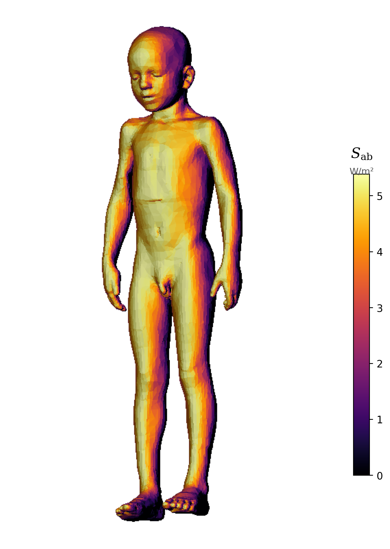
Absorbed power density \(S_{\mathrm{ab}}\) rendered on the Thelonious phantom at 28 GHz.
Next steps
- Tutorial 2: Fidelity levels and convergence: the nine-level hierarchy,
sweep_levels, comparison plots - Tutorial 3: Tissue physics and Fresnel transmission: Cole-Cole model, Fresnel transmission, level 3 vs level 2
- Tutorial 4: ICNIRP 2020 compliance: regulatory limits, compliance evaluation, power sweeps
- Tutorial 5: Coherent MIMO and ECBF: field channel, exposure operator, exposure-constrained beamforming