Coherent MIMO dosimetry
For a step-by-step walkthrough with code, see the coherent MIMO tutorial.
Levels 7 and 8 extend AEGIS to coherent multi-antenna systems. Instead of scalar power per path, these levels use complex polarization-amplitude vectors and antenna element structure to compute the interference pattern on the body surface.
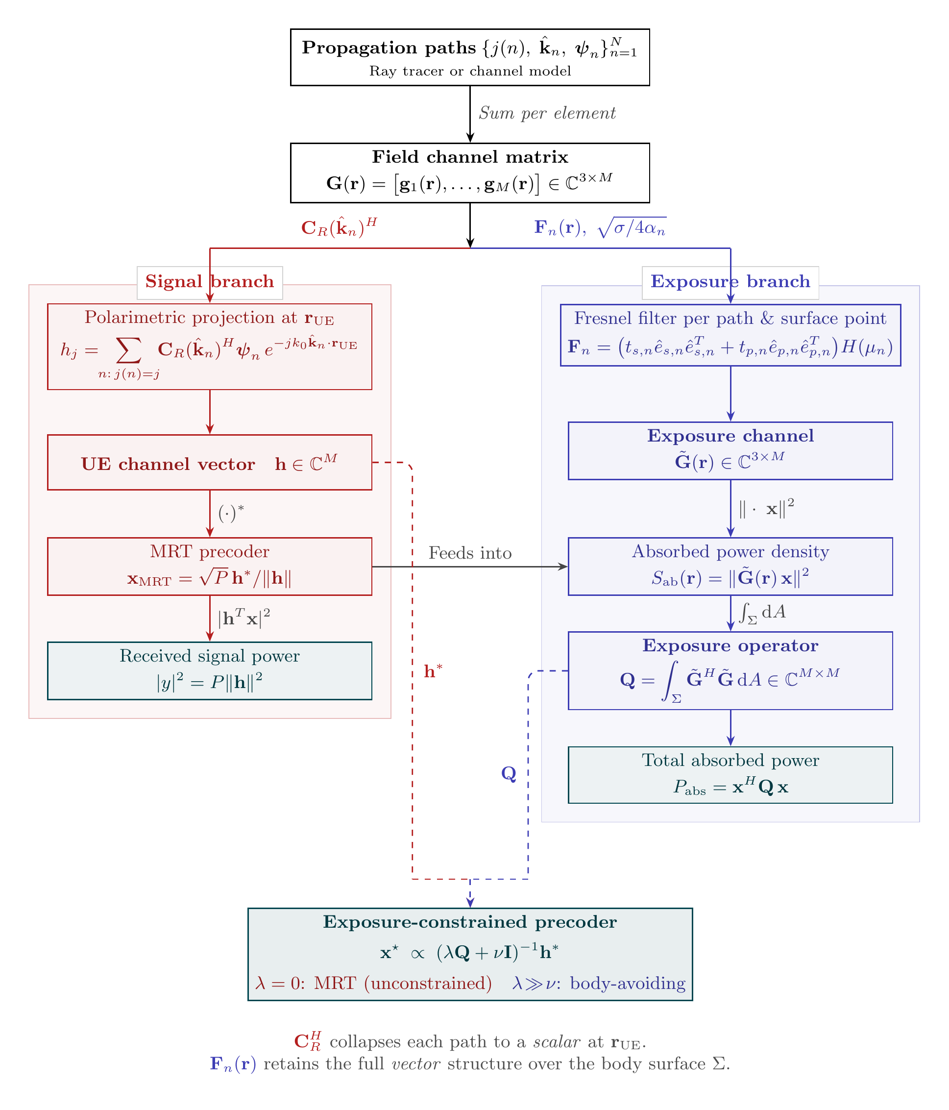
Signal branch (red) and exposure branch (blue) of the coherent MIMO pipeline.
From incoherent to coherent
Incoherent dosimetry (Levels 0-6) sums power contributions independently:
Coherent dosimetry (Level 7) sums complex field contributions, then takes the squared magnitude:
where \(\tilde{\mathbf{G}}(\mathbf{r})\) is the body-surface channel matrix and \(\mathbf{x}\) is the precoding vector.
The difference matters when paths from the same antenna element can interfere constructively or destructively on the body surface.
PropagationPaths for coherent use
Coherent levels need the full PropagationPaths object with complex polarization-amplitude vectors psi and an element_index array mapping each path to its originating antenna element. The psi vectors carry both polarization direction and amplitude, with \(S_i = |\boldsymbol{\psi}_i|^2 / (2 Z_0)\) giving the per-path power density. The tutorial shows how to construct these paths from scratch.
The body-surface channel
The coherent pipeline builds \(\tilde{\mathbf{G}}(\mathbf{r})\) in three steps:
-
TE/TM decomposition - For each (triangle, path) pair, compute the TE and TM basis vectors and the Fresnel transmission operator \(\mathbf{F}_n(\mathbf{r})\).
-
Depth coupling - Apply a factor \(\sqrt{\sigma / 4\alpha}\) that accounts for the exponential decay of the field into tissue.
-
Element accumulation - Sum path contributions by antenna element to produce a \((3 \times M_{\mathrm{ant}})\) matrix at each triangle.
Two approximations make this tractable:
- Approximation 1 (TM direction): treats the refracted TM direction as parallel to the incidence plane projection onto the surface. Error \(\leq\) 4%.
- Approximation 2 (depth coupling): uses a universal depth coupling factor independent of incidence angle. Error \(\leq\) 0.44%.
Exposure operator Q
The exposure operator integrates the squared-norm field over the body surface:
where \(a_m\) is the area of triangle \(m\). Key properties:
- \(\mathbf{Q}\) is Hermitian and positive semi-definite
- \(P_{\mathrm{abs}} = \mathbf{x}^H \mathbf{Q} \mathbf{x}\) for any precoding vector \(\mathbf{x}\)
- Its eigenvalues tell you the worst-case and best-case absorption for unit-power precoders
# After a Level 7 computation
result = engine.compute(body, paths, level=7, precoder=precoder, h=h)

Q = result.Q                  # (M_ant, M_ant) Hermitian PSD
evals = result.eigenvalues    # descending order
print(f"Worst-case P_abs: {evals[0]:.4f} W (for unit power)")
print(f"Best-case P_abs: {evals[-1]:.6f} W")
Exposure-signal alignment
The metric \(\rho\) quantifies how aligned the communication channel \(\mathbf{h}\) is with the exposure eigenvectors:
\(\rho = 1\) means MRT beamforming hits the worst-case exposure direction. \(\rho \approx 0\) means the channel is nearly orthogonal to the dominant exposure mode, so MRT is already low-exposure.
Precoders
The Precoder class wraps a complex precoding vector \(\mathbf{x}\). Use Precoder.mrt(h, P=1.0) for maximum ratio transmission (\(\mathbf{x} = \sqrt{P}\,\mathbf{h}^* / \|\mathbf{h}\|\)) or Precoder.ecbf(h, Q, P_abs_max, P) for exposure-constrained beamforming. The tutorial demonstrates both precoders with worked examples.
Level 7: coherent map
Computes \(S_{\mathrm{ab}}(\mathbf{r})\), \(\mathbf{Q}\), eigenvalues, and \(\rho\) for a given precoder. Pass level=7 with a Precoder and optionally h to get the exposure-signal alignment metric. See the tutorial for a full worked example.
Corollary 4.1
For a single plane wave (one path, one element), Level 7 matches incoherent Level 3 within 10%. This validates the coherent pipeline against the simpler incoherent computation.
Corollary 4.2
Averaging Level 7 over many random phase realizations converges to the incoherent result. This confirms that incoherent dosimetry is the expected value of coherent dosimetry.
Level 8: ECBF
Level 8 solves a QCQP to find the precoder maximizing signal power subject to an absorption constraint:
The solver works in the Q eigenbasis and finds the optimal Lagrange multiplier via bisection. When the MRT precoder already satisfies the constraint, ECBF returns MRT (it is the unconstrained optimum). The tutorial compares MRT and ECBF side by side with a worked example.