Geometry and mesh operations¶

AEGIS operates on triangle meshes representing the human body surface. The geometry module handles mesh loading, projected area computation, directivity analysis, ambient occlusion, and ICNIRP spatial averaging.

BodyMesh¶

The BodyMesh dataclass stores a triangle mesh as four arrays:

import aegis

body = aegis.BodyMesh.load("thelonious.stl")
print(f"{body.n_triangles} triangles")
print(f"Total area: {body.total_area:.4f} m²")
print(f"Bounding box diagonal: {body.scale:.3f} m")

BodyMesh is a frozen dataclass. All arrays are read-only after construction.

Loading STL files¶

AEGIS reads binary STL format. The loader recomputes degenerate normals from vertex cross products and normalizes all normals to unit length.

from aegis.geometry import load_stl_binary, triangle_areas

vertices, normals, centroids = load_stl_binary("thelonious.stl")
areas = triangle_areas(vertices)

Synthetic meshes¶

BodyMesh.from_arrays() builds a mesh from raw vertex arrays, computing centroids, areas, and optionally normals automatically:

import numpy as np

# Flat square as two triangles
vertices = np.array([
    [[0, 0, 0], [1, 0, 0], [1, 1, 0]],
    [[0, 0, 0], [1, 1, 0], [0, 1, 0]],
], dtype=float)

body = aegis.BodyMesh.from_arrays(vertices, name="square")

If you need explicit control over normals, pass them as the second argument. Otherwise they are computed from the vertex cross product.

For full manual construction (all four arrays):

normals = np.array([[0, 0, 1], [0, 0, 1]], dtype=float)
centroids = vertices.mean(axis=1)
areas = triangle_areas(vertices)

body = aegis.BodyMesh(
    vertices=vertices, normals=normals,
    centroids=centroids, areas=areas, name="square",
)

Projected area¶

The projected area \(A_\perp(\hat{k})\) is the cross-sectional area of the body as seen from direction \(\hat{k}\):

Only front-facing triangles contribute (the ReLU ensures back-facing triangles are excluded).

from aegis.geometry import compute_projected_area, fibonacci_sphere

# Sample 256 directions uniformly on the sphere
k_dirs = fibonacci_sphere(256)
A_perp = compute_projected_area(body.normals, body.areas, k_dirs)

print(f"Mean A_perp: {A_perp.mean():.4f} m²")
print(f"Max A_perp: {A_perp.max():.4f} m²")

Cauchy formula¶

For a convex body, the mean projected area over all directions equals one-quarter of the total surface area:

This is the Cauchy formula. It holds for all closed surfaces, convex or not. The compute_projected_area function computes the sum without visibility testing, so it obeys Cauchy exactly. For the true silhouette area (with self-occlusion), the value would be smaller.

from aegis.geometry import cauchy_projected_area, mean_projected_area, cauchy_relative_error

A_cauchy = cauchy_projected_area(body.total_area)
A_mean = mean_projected_area(A_perp)
error = cauchy_relative_error(A_perp, body.total_area)

print(f"Cauchy: {A_cauchy:.4f} m², Mean: {A_mean:.4f} m²")
print(f"Relative error: {error:.2%}")

Directivity¶

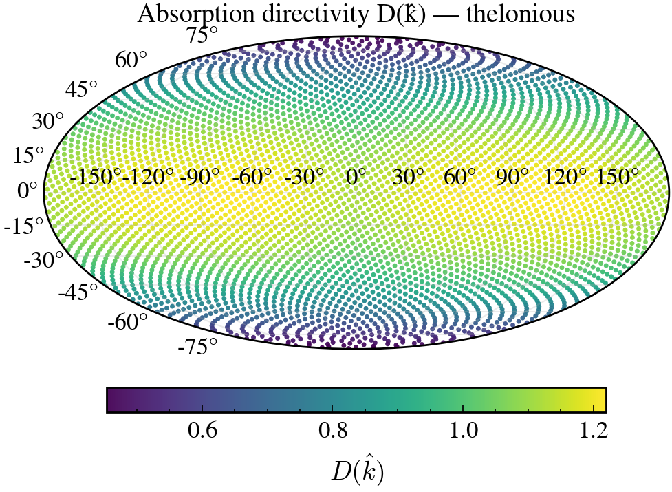
Absorption directivity \(D(\hat{k})\) of the Thelonious phantom on a Mollweide projection.

Directivity \(D(\hat{k})\) normalizes the projected area so that its mean over the sphere equals 1:

Used by Level 1 to weight contributions from different directions without computing the full spatial map.

from aegis.geometry import compute_directivity

D = compute_directivity(A_perp)
print(f"D range: [{D.min():.2f}, {D.max():.2f}]")
print(f"D mean: {D.mean():.4f}")  # 1.0 by construction

Spherical harmonics compression¶

For fast evaluation, directivity can be compressed into spherical harmonic (SH) coefficients:

from aegis.geometry import fit_sh, eval_sh, sh_reconstruction_error, spherical_angles_from_k_hat

theta, phi = spherical_angles_from_k_hat(k_dirs)

# Fit at degree L=8 (81 coefficients)
coeffs = fit_sh(D, theta, phi, L=8)
D_reconstructed = eval_sh(coeffs, theta, phi, L=8)

# Check reconstruction quality
metrics = sh_reconstruction_error(D, theta, phi, L=8)
print(f"RMS error: {metrics['rms']:.4f}")
print(f"Max error: {metrics['max_abs']:.4f}")

For a typical human body mesh, \(L = 4\) (25 coefficients) gives sub-1% RMS error. \(L = 8\) is essentially exact.

Ambient occlusion¶

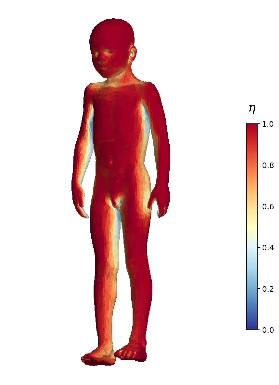
Ambient occlusion factor \(\eta\) on the Thelonious phantom. Red regions are fully exposed, blue regions are self-shadowed.

The exposure fraction \(\eta(\mathbf{r})\) measures how much of the hemisphere above each triangle is visible (not blocked by other body parts). AEGIS computes this via BVH-accelerated cosine-weighted ray tracing. When Numba is installed, the BVH traversal and ray-triangle intersection are JIT-compiled for 50-100x speedup on large meshes.

from aegis.geometry import compute_ambient_occlusion

eta = compute_ambient_occlusion(body, n_rays=64, seed=0)
print(f"eta range: [{eta.min():.2f}, {eta.max():.2f}]")

A triangle on the top of the head has \(\eta \approx 1.0\) (fully exposed). A triangle in the armpit might have \(\eta \approx 0.3\) (mostly occluded).

Spatial averaging¶

ICNIRP 2020 Table 2 specifies that \(S_{\mathrm{ab}}\) must be averaged over a square 4 cm\(^2\) surface area for compliance assessment. The basic restriction for general public exposure above 6 GHz is 20 W/m\(^2\) (not 10, which is the \(S_{\mathrm{inc}}\) reference level from Table 5).

The engine computes spatial averaging automatically using a precomputed sparse matrix \(\mathbf{G}\):

where \(\mathbf{G}\) is a row-stochastic \((M \times M)\) matrix encoding the 4 cm\(^2\) neighborhood structure. Each row \(i\) contains area-weighted contributions from the triangles nearest to triangle \(i\), accumulated until the total area reaches 4 cm\(^2\).

result = engine.compute(body, paths, mode="spatial")

# Spatial averaging is always-on. No flag needed.
print(f"Peak raw S_ab: {result.peak_sab:.2f} W/m²")
print(f"Peak averaged S_ab: {result.peak_sab_averaged:.2f} W/m²")
print(f"Compliant: {result.compliant_sab}")

You can also use the averaging matrix directly:

from aegis.geometry import precompute_averaging_matrix

G = precompute_averaging_matrix(body.centroids, body.areas, target_area_m2=4e-4)
sab_avg = G @ result.sab

The matrix \(\mathbf{G}\) depends only on mesh geometry, not on \(S_{\mathrm{ab}}\). Precompute it once per body mesh and reuse across evaluations. The engine caches it internally.

For JAX-based optimization, convert \(\mathbf{G}\) to a dense JAX array:

from aegis.geometry.averaging import averaging_matrix_to_jax

G_jax = averaging_matrix_to_jax(G)
sab_avg = G_jax @ sab  # differentiable