Overview
AEGIS computes absorbed power density on human body meshes. Two APIs are available. Use level= (0-8) to select a predefined fidelity level by integer. Use mode= (bound, aggregate, spatial, coherent, ecbf) with optional correction flags when you need finer control over which physics are applied. Both call the same kernels. See fidelity levels for the full mapping.
Physical model
At mmWave frequencies (above 6 GHz), the skin depth in human tissue is 0.3 to 0.5 mm. All incident power is absorbed in the outermost layer. Absorption is a surface phenomenon, not a volumetric one, which eliminates the need for full-wave simulation of the body interior.
The core equation computes absorbed power density at each point \(\mathbf{r}\) on the body surface:
\(S_{\mathrm{inc}}\) is the incident power density of the incoming wave. \(T_0\) is the normal-incidence Fresnel power transmission into tissue, a single scalar that captures the material response. \(\hat{n}(\mathbf{r})\) is the outward surface normal at point \(\mathbf{r}\), and \(\hat{k}\) is the wave propagation direction. The \([\cdot]_+\) operator (ReLU) enforces that only illuminated surface patches absorb power: triangles facing away from the wave contribute zero.
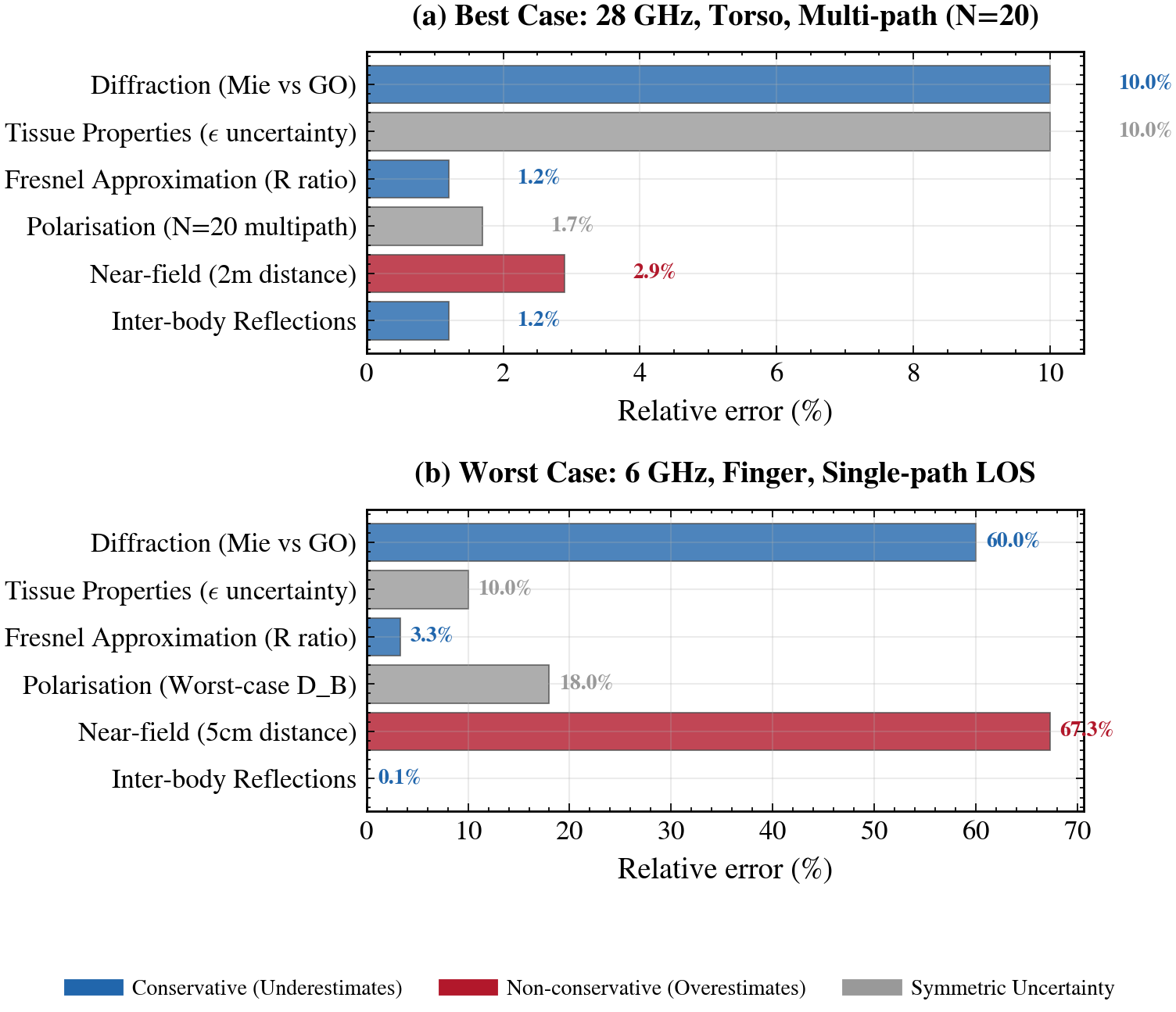
Relative error contributions by source. Best case (28 GHz torso, multipath) vs worst case (6 GHz finger, single path).
The framework rests on three assumptions. Each incoming path is a plane wave at the body (far-field). Each mesh triangle is locally flat (flat-facet approximation). The tissue beneath each triangle behaves as a semi-infinite lossy dielectric (half-space Fresnel model).
These assumptions break down in a few regimes. At near-field distances (less than a few wavelengths from the source), the plane-wave assumption fails. Below 6 GHz, skin depth grows and absorption becomes volumetric. On high-curvature regions like fingers and ears, the flat-facet approximation loses accuracy when triangle size approaches the wavelength.
The geometric framework matches the full Fresnel solution to within 0.35% for typical body geometries. AEGIS validates this against the analytical Mie sphere solution across body part sizes and frequencies. For full derivations, see the monograph in theory/.
Typical workflow
- Load a tissue model (skin properties at your frequency)
- Load a body mesh (triangle mesh in STL format)
- Define propagation paths (directions and powers, or full complex amplitudes from a ray tracer)
- Run the engine with your chosen mode and corrections
- Inspect the result (per-triangle S_ab, total P_abs, compliance status)
For coherent and ECBF modes, you also provide a precoding vector (via Precoder.mrt()) and optionally a UE channel vector h.
Key outputs
result.sab- per-triangle absorbed power density [W/m\(^2\)]result.p_abs- total absorbed power [W]result.peak_sab- maximum \(S_{\mathrm{ab}}\) across all trianglesresult.sar_wb- whole-body SAR [W/kg] (if body mass provided)result.compliant_sab- True/False if spatial averaging was applied, None otherwiseresult.Q- exposure operator (coherent and ECBF modes)result.eigenvalues- Q eigenspectrum (coherent and ECBF modes)result.rho- exposure-signal alignment (coherent and ECBF modes)
See fidelity levels for details on each mode and correction.
Comparing fidelity levels
sweep_levels() runs multiple fidelity levels in one call and returns a dict of results. Levels that need unavailable parameters (e.g. \(A_{\mathrm{ab}}\) for level 0) are silently skipped.
results = engine.sweep_levels(body, paths)
for level, r in results.items():
    print(f"Level {level}: peak = {r.peak_sab:.2f} W/m², P_abs = {r.p_abs:.4f} W")
To quantify the differences between results, use DosimetryResult.compare():
from aegis import DosimetryResult

comparison = DosimetryResult.compare(
    {f"L{k}": v for k, v in results.items()}
)
print(f"Relative errors: {comparison['relative_error']}")
This returns peak \(S_{\mathrm{ab}}\), \(P_{\mathrm{abs}}\), pairwise RMSE, max absolute error, and relative error across all pairs.
Scaling and compliance shortcuts
DosimetryResult.scale(factor) returns a new result with all power quantities scaled. Combined with evaluate_compliance(), this lets you sweep transmit power without rerunning the engine:
result = engine.compute(body, paths, mode="spatial")

# Scale to 2 W and check compliance
scaled = result.scale(2.0)
compliance = scaled.evaluate_compliance()
print(f"Compliant at 2 W: {compliance.overall_pass}")
See compliance for the full compliance workflow including max_compliant_power().
Serialization
Both PropagationPaths and DosimetryResult support round-trip serialization:
# Save
d = result.to_dict()
s = result.to_json(indent=2)

# Load
result2 = DosimetryResult.from_dict(d)
result3 = DosimetryResult.from_json(s)
PropagationPaths has the same to_dict() / from_dict() pattern. Complex arrays (psi, Q, eigenvalues) are serialized as {"real": [...], "imag": [...]}.