Tissue and Fresnel transmission
For a step-by-step walkthrough with plots, see the tissue and Fresnel tutorial.
AEGIS models the electromagnetic properties of human tissue to compute how much incident power is absorbed at the body surface. The tissue module provides dielectric models, Fresnel transmission coefficients, and a database of tissue properties from the IT'IS foundation.
Dielectric properties
At mmWave frequencies, tissue behaves as a lossy dielectric characterized by two parameters: relative permittivity \(\varepsilon_r\) and conductivity \(\sigma\). These combine into a complex refractive index:
For skin at 28 GHz: \(\varepsilon_r = 17.0\), \(\sigma = 25.0\) S/m, giving \(|\tilde{n}| \approx 4.84\).
TissueModel
The TissueModel dataclass wraps dielectric parameters and provides derived quantities. Create one with TissueModel.from_params() or use the predefined constants. The tutorial covers creation and usage in detail.
Predefined tissues
Four tissue types are hardcoded from published literature:
| Tissue | Frequency | \(\varepsilon_r\) | \(\sigma\) (S/m) | \(T_0\) |
|---|---|---|---|---|
SKIN_28GHZ | 28 GHz | 17.0 | 25.0 | 0.539 |
SKIN_60GHZ | 60 GHz | 7.9 | 36.4 | 0.623 |
MUSCLE_28GHZ | 28 GHz | 25.0 | 30.0 | 0.493 |
FAT_28GHZ | 28 GHz | 4.0 | 2.0 | 0.876 |
IT'IS database
For arbitrary tissue types and frequencies, AEGIS uses the IT'IS v5.0 database with a 4-pole Cole-Cole model (Gabriel 1996). Call TissueModel.from_database("Skin", 28e9) with any tissue name from the IT'IS database. The database file (itis_v5.db) ships in data/ inside the repo. Override with AEGIS_DATA_DIR if needed.
The Cole-Cole model computes complex permittivity from 14 parameters (4 poles with relaxation times spanning picoseconds to milliseconds). This gives accurate dielectric properties across 10 Hz to 100 GHz.
Fresnel transmission
The fraction of incident power that enters the tissue depends on the angle of incidence \(\theta_i\). AEGIS computes Fresnel power transmission coefficients for both TE and TM polarizations.
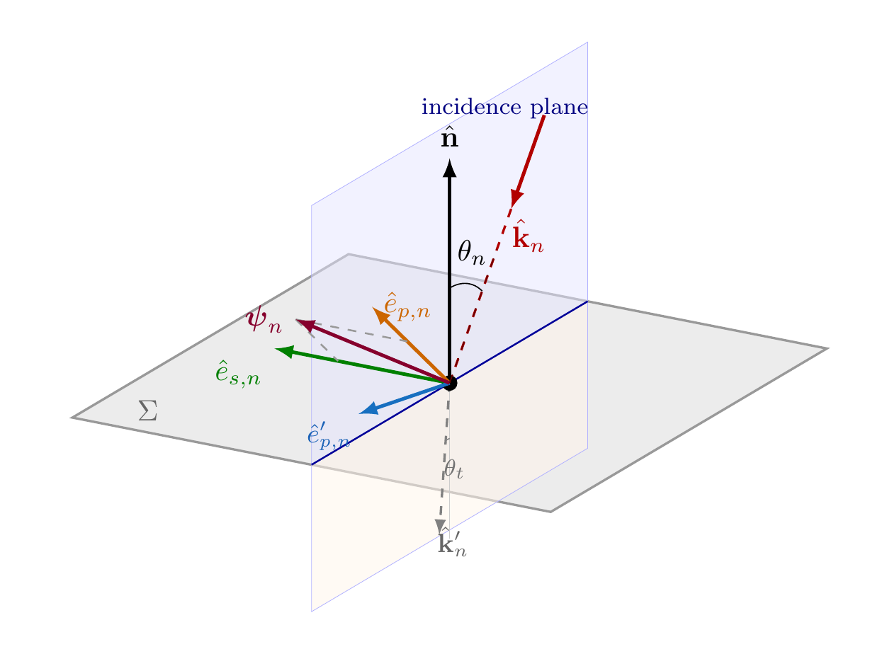
Incidence plane geometry showing surface normal \(\hat{n}\), wave vector \(\hat{k}\), and TE/TM polarization basis vectors.
Normal incidence
At normal incidence (\(\theta_i = 0\)), the transmission coefficient simplifies to:
This is the single most important tissue parameter. For skin at 28 GHz, \(T_0 = 0.539\), meaning 53.9% of incident power is absorbed.
Angle-dependent transmission
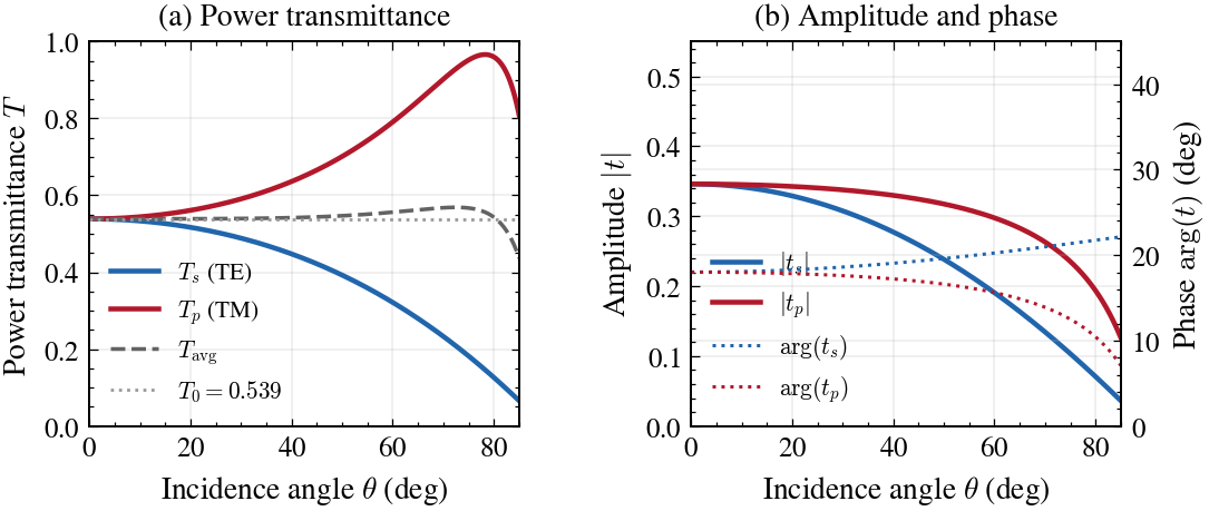
Power transmittance and amplitude coefficients for skin at 28 GHz.
For oblique incidence, TE and TM polarizations transmit different fractions. fresnel_transmission(mu, n_tilde) returns both \(T_s\) (TE) and \(T_p\) (TM) power transmission coefficients. TM polarization always transmits more than TE at oblique angles, which matters at Level 4 and above where polarization corrections are applied. The tutorial plots the full angular dependence and demonstrates the pseudo-Brewster compensation effect.
The unpolarized (average) transmission is:
Amplitude coefficients
Coherent dosimetry (Levels 7-8) needs complex amplitude transmission coefficients, not power. Use fresnel_amplitude(mu, n) for this. The power coefficient relates to the amplitude as \(T = \text{Re}(\xi) / \mu \cdot |t|^2\) where \(\xi\) is the normal wave-vector component in tissue.
How fidelity levels use tissue
| Level | Tissue parameter | Notes |
|---|---|---|
| 0-2 | \(T_0\) (scalar) | Same transmission for all angles |
| 3 | \(T_{\mathrm{avg}}(\theta)\) | Angle-dependent, unpolarized |
| 4 | \(T_s, T_p\) separately | Polarization-resolved |
| 5-6 | \(T_{\mathrm{avg}}(\theta)\) + curvature | Physical optics correction |
| 7-8 | \(t_s, t_p\) (complex amplitudes) | Full coherent Fresnel operator |
The transition from Level 2 to Level 3 (replacing constant \(T_0\) with angle-dependent \(T_{\mathrm{avg}}\)) changes total absorbed power by about 0.35% on typical body meshes. The correction matters more for geometries with many grazing-incidence triangles.